Inspecting velocities

This example will inspect the calculated velocities.

Note

The velocities are calculated from the distance so it is a bit noisy.

• 
• 
• 

import matplotlib.dates as mdates
import seaborn as sns
from matplotlib import pyplot as plt

from gpxplotter import plot_filled, read_gpx_file
from gpxplotter.common import cluster_velocities

sns.set_context("notebook")

for track in read_gpx_file("example1.gpx"):
    for i, segment in enumerate(track["segments"]):
        fig, (axi, axj) = plt.subplots(
            constrained_layout=True, ncols=2, figsize=(10, 5)
        )
        # First draw a histogram:
        sns.histplot(
            x=segment["velocity"],
            ax=axi,
            stat="density",
            kde=True,
            line_kws={"label": "kde", "lw": 3},
        )
        axi.set_title("Histogram of velocities", loc="left")
        axi.set(xlabel="Velocity / m/s", ylabel="Frequency")
        axi.legend(frameon=False)
        # Add clustering of velocities for grouping them into levels:
        level = cluster_velocities(segment["velocity"], n_clusters=6)
        scatter = axj.scatter(
            segment["time"], segment["velocity"], c=level, cmap="viridis"
        )
        axj.legend(
            *scatter.legend_elements(num=len(set(level))),
            title="Velocity level",
        )
        axj.xaxis.set_major_formatter(mdates.DateFormatter("%H:%M:%S"))
        axj.tick_params(axis="x", rotation=25)
        axj.set(xlabel="Time", ylabel="Velocity")
        sns.despine(fig=fig)
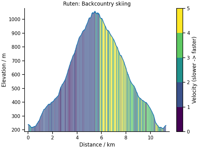
        # The velocity levels is also calculated when loading the gpx-file:
        fig2, _ = plot_filled(
            track,
            segment,
            xvar="Distance / km",
            yvar="elevation",
            zvar="velocity-level",
        )
        sns.despine(fig=fig2)
        # The number of levels can be changed by updating the
        # velocity-level:
        levels = cluster_velocities(segment["velocity"], n_clusters=6)
        if levels is not None:
            segment["velocity-level"] = levels
        fig3, _ = plot_filled(
            track,
            segment,
            xvar="Distance / km",
            yvar="elevation",
            zvar="velocity-level",
            cmap="viridis",
            color="k",
        )
        sns.despine(fig=fig3)
plt.show()